CJob Quickstart

This document is intended to be a quick primer/refresh on using the CJob GUI to create jobs for the Vistec. For some useful examples of basic jobs, look in the Examples subdirectory of your job folder.

Starting CJob

1. There are a number of ways to start CJOB. On the CAD computer (either locally or via a VNC session) it can be started by typing cjob in a terminal window or picking CJob from the main desktop menu. On the EBPG computer, it can be run either from a terminal (the cjob command again) or the desktop icon.
   
   
2. If using the EBPG computer, make sure you switch into your environment before running CJob from a terminal window. The command ce <username> is used to do this.
   
   
3. If you don’t want to lock up the terminal window while CJOB is running, execute it in the background by typing cjob& instead of cjob .
   
   

Creating Basic Jobs

1. When you open up CJob, you’ll see a screen that looks (intentionally) similar to the LayoutBEAMER? interface.
   
   
   
   
2. Every job created in CJob starts with a Substrate object. Drag and drop a Substrate box into the white process-flow area. A dialog will pop up allowing you to select the substrate type and give it a name.
   
   
   
   
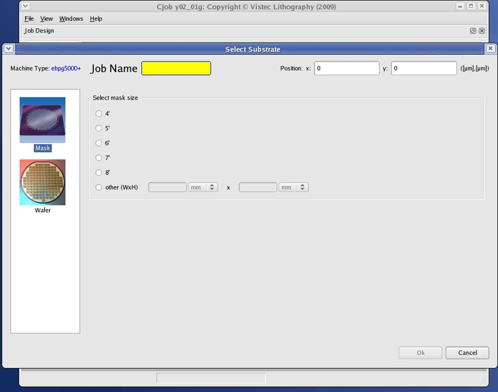
   1. It is EXTREMELY important not to use a name with spaces in it. CJob will allow it but it will cause an error when you try to execute the job or reopen the .cjob file. All other non-wildcard characters are fine.
      
      
   2. For piece parts, define the substrate as a mask plate with arbitrary dimensions and just enter the height and width in millimeters.
      
      
3. The substrate boundaries tell the system where to write; it won’t let you add exposure features outside the substrate boundary. It serves no other real purpose, so when in doubt just choosing a substrate larger than your actual substrate is fine.
   
   
4. Substrate objects must be connected to Exposure objects. Each Exposure object in a job flow exports to a different executable file, so if you had (for example) a three-layer write with processing in between each layer, you could connect three Exposure objects (one for each layer) to a single Substrate object.
   
   
5. To connect an object to another object, drag and drop it just below the object you want to connect it to (the mouse cursor will change when you can make a connection).
   
   
6. Once the Exposure object is in place, a dialog box will pop up as it did with the substrate object. Here you can give the exposure a name (again, no spaces!) and specify exposure-level options like height checking.
   
   
   
   
7. Global alignment markers are defined in the Exposure object, but since the coordinates are given relative to the center of the exposure and there aren’t any objects in the exposure yet, it’s easiest to come back and set these up later (see the section on aligned writes).
   
   
8. An Exposure object needs things to expose. There are three exposable object types in CJob: Pattern, Shape, and Identifier, as well as a separate container object called Layout that can be used to set up arrays and other complex sequences of patterns. Any and all of these can be connected to the Exposure object by dragging and dropping, either within the Exposure dialog box or on the main screen.
   
   
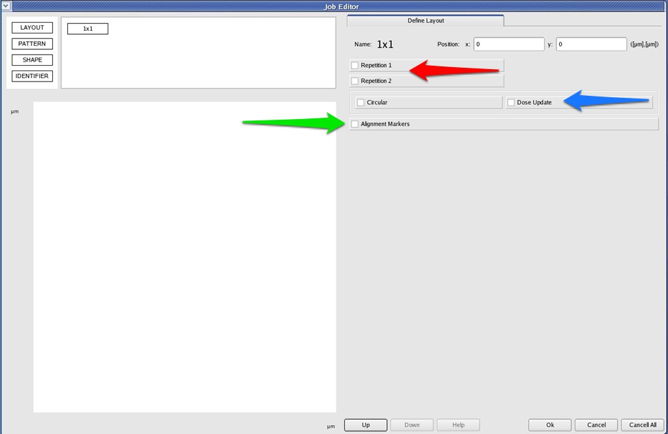
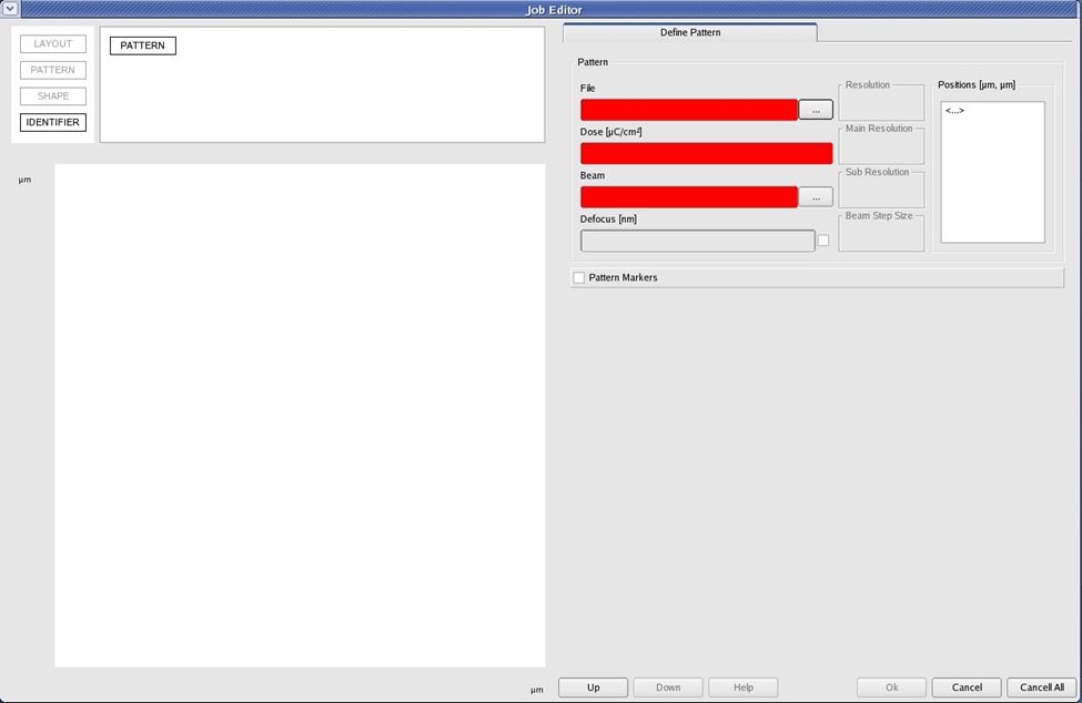
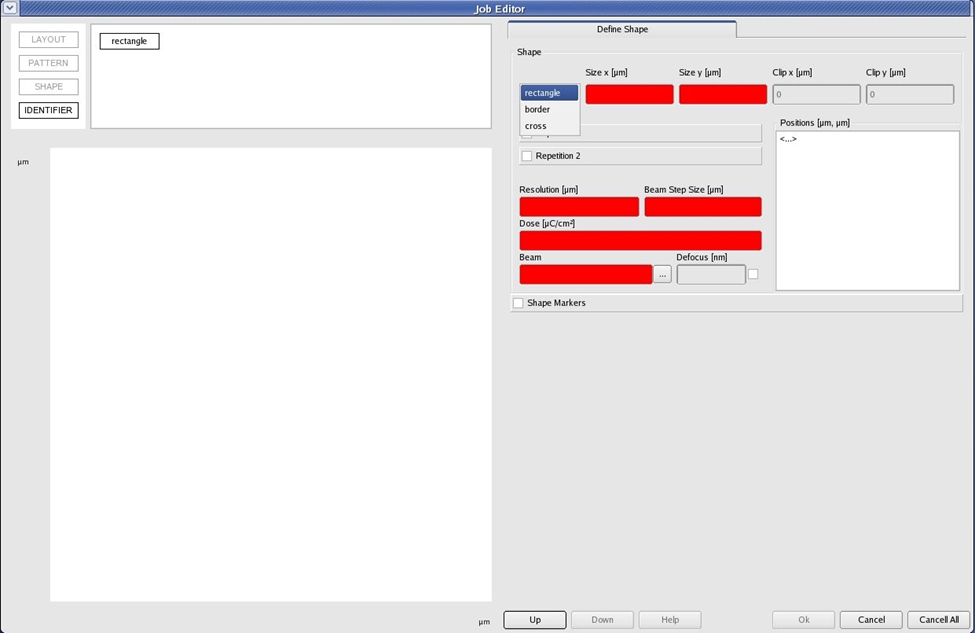
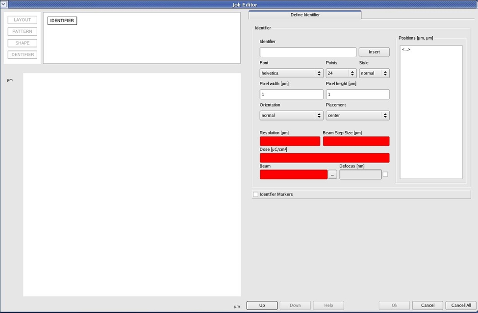
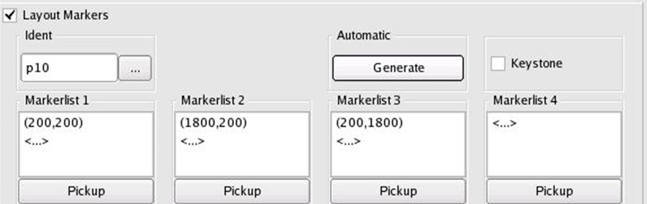
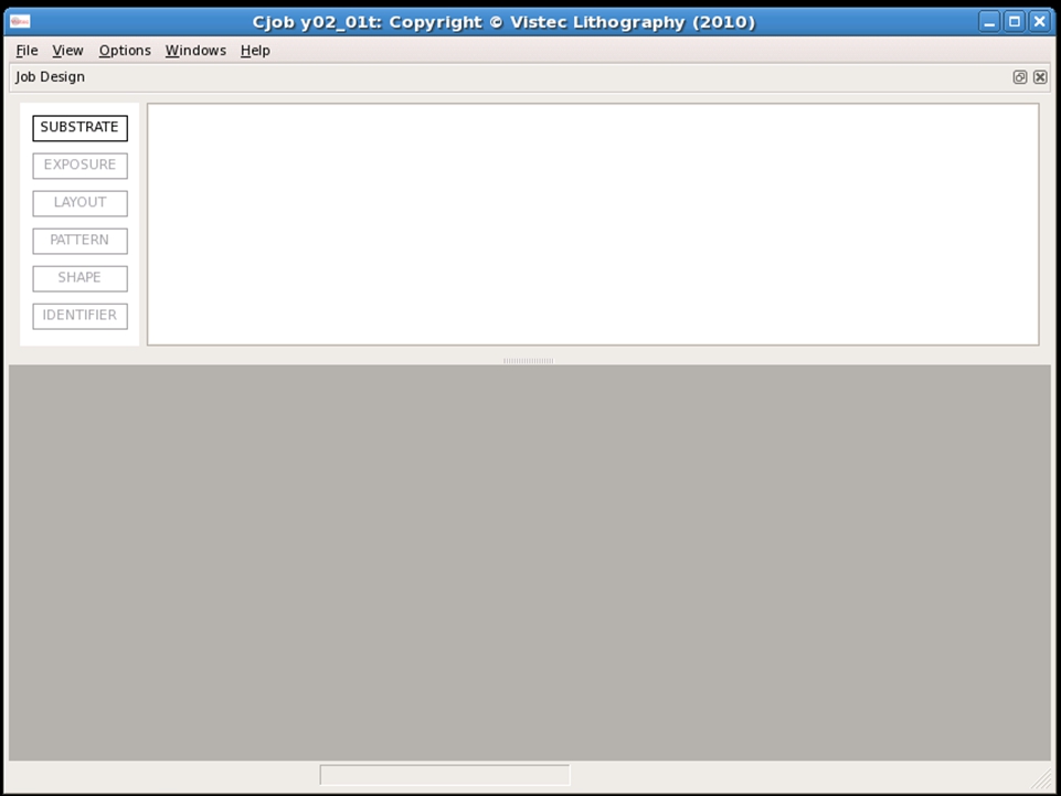
   1. Each of these objects has specific properties that are discussed later in this guide in more detail
      
      
   2. A completed job flow will consist of a single Substrate object connected to one or more Exposure objects, each of which may have any number of Layout, Pattern, Shape, or Identifier objects connected to it.
      
      

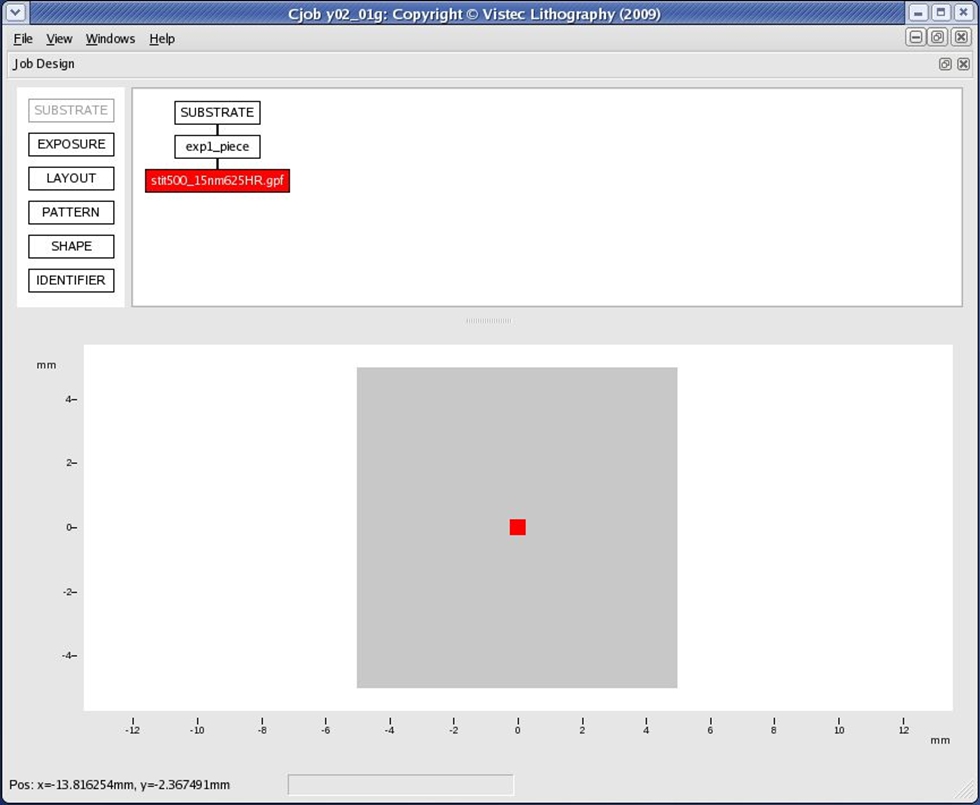
      The main window with a simple job flow defined. Here a Substrate object called SUBSTRATE is connected to an Exposure object called exp1_piece, which is connected to a Pattern object containing a GPF file called stit500_15nm625HR.gpf. The substrate, with the pattern in the center of it, is displayed in the lower window.

      
      
9. In order to generate an executable .job file, the job has to be exported. This is done using the Export Job option in the file menu, also reachable with the CTRL+J shortcut.
   
   
   1. The Save Job option will NOT save an executable .job file, just a .cjob file containing the flow you’ve set up in case you want to edit it in CJob later. Files with the .cjob extension can’t be executed and can only be edited with CJob
      
      
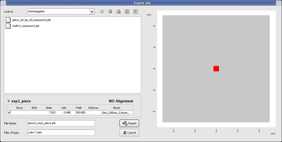
10. The Export dialog box (see below) will give you a list of all Exposure objects in the design flow and allow you to choose which one to export. By default, exports will be saved in the /jobs subfolder of your home directory. CJob gives exports filenames of the type substratename_exposurename.job by default, but this can be changed to whatever you want.
    
    
    
    
11. After exporting each Exposure object you want to expose (you can pick another after you’ve exported one), close the Export dialog box with the Done/Cancel button.
    
    

Advanced Operation

Layout Object

The Layout object is an all-purpose container update that lets you greatly expand the flexibility of your CJOB jobs. It consists of a set of instructions for how and where to expose any number of Pattern, Shape, Identifier, or even other Layout objects attached to it.

1. The Layout object must be attached to either an Exposure or Layout object in the flow to work. Dragging a Layout object into the job flow chart will bring up the dialog box below
   
   

   The Layout dialog box. The red arrow indicates the section where exposure arrays can be set up, the blue arrow indicates the Dose Update setting that allows the dose to be varied between array elements, and the green arrow indicates where Layout-level alignment marks can be added.

   
   
2. The most useful thing you can do with a Layout object is set up exposure arrays of sub-objects. This is done using the Repetition 1 and Repetition 2 checkboxes; check one to do a 1D array and check both to do a 2D array. When checked, the Repetition boxes expand to look like this:
   
   

   Close-up of the expanded Repetition settings in the Layout dialog box. In this case, a 5x5 2D repetition of a pattern that is 500x500 μm wide is set up, with 100 μm of space between adjacent patterns in both the X and Y directions.

   
   
   1. In each Repetition box, there are several numbers that need to be entered:
      
      
      1. Count refers to the number of elements in each repetition of the array.
         
         
      2. Vector is the width or height of the pattern or other object being repeated
         
         
      3. Spacing is the space between adjacent elements in the array.
         
         
   2. Some tips when setting up repetition arrays:
      
      
      1. The system calculates the center-center distance (pitch) of adjacent array elements by adding the Vector and Spacing variables. So in figure 7, a Vector of 300 μm and a spacing of 300 μm would give the same results as the numbers used. I like to think in terms of pitch, so I generally input the pitch of my array as the Vector value and leave the Spacing value at zero.
         
         
      2. Arrays generally are, but do not have to be, orthogonal. You could, for example, set up a single repetition axis to be spaced 100 μm in x and 100 μm in y between elements, which would give you a diagonal line of features. This feature is of questionable utility but may come in handy in certain situations.
         
         
3. The Circular option in the Layout box is useful if you need to cover a wafer or other circular surface with a pattern. Simply enter the radius of your circle (100mm for a 4” wafer, for example), choose NET or GROSS filling (NET filling will ignore array elements that fall only partially on the circle, while GROSS will fill in as much of them as possible), and specify whether the circle origin is the center of the substrate or the local center of the Layout object. Object sizes and spacings are still set in the Repetition boxes as before.
   
   
4. The Dose Update option is important, as you’ll often want to do an array of features with varying doses to find the best electron dose to use for a particular pattern. Checking the Dose Update box gives the options shown in figure 8:
   
   

   The Dose Update dialog. Here the user has set the dose to increase by 10 μC/cm2 for each successive array element.

   
   
   1. The far-left drop-down box lets you choose the dose operator ; i.e. whether you want to add, subtract, multiply, or divide the dose from element to element. The number to the left of it is the coefficient; in the case of Figure 8, the user has chosen to add 10 μC/cm2 to the dose at each array element.
      
      
      1. It should be noted that the relationship between dose and resist develop rate is exponential, which means a logarithmic dose array is more likely to give you good results. For example, multiplying the dose by 5-10% (1.05 or 1.1) per element will usually give a good spread.
         
         
   2. You can choose to update the dose either on Scan Order (every element), or just Repetition 1 or 2. If you chose to update on Repetition 1, for example, and your settings were the ones in figure 7, all the elements in each row would have the same dose, which would increase every row. In most cases, you’ll want to update on Scan Order.
      
      
5. Finally, alignment markers can be added for the Layout object (if you have an array of patterns you want to align to a single set of marks, for example). The details of doing this are covered in the section on alignment marks.
   
   

Pattern Object

The Pattern object is the module that lets you expose a GPF-format pattern. It is usually, but not always, connected to a Layout object that sets up positioning, array, and other placement settings for it.

1. To place a Pattern object, drag it onto the job flow and connect it to either a Layout or Exposure object. The dialog below will appear when the module is placed.
   
   

   The Pattern dialog box. The options here allow you to select the pattern file, the exposure dose, the beam current, and an optional beam-defocus width, as well as an offset position if desired.

   
   
2. The three major settings here are File, Dose, and *Beam*
   
   
   1. File is the filename of the GPF (pattern) file you want to expose. Click the button next to the entry box to bring up a dialog that will allow you to browse for the file you want to expose. Note that if you remembered to change environments before starting up CJOB, this dialog will start in your /jobs directory on the EBPG computer by default.
      
      
   2. Dose is the areal electron dose (in μC/cm2) that you want to expose the pattern at. Note that if you set up a dose array with this Pattern object, the dose you set here will be the array’s starting dose.
      
      
   3. Beam is the file corresponding to the beam current you want to expose at. Clicking the browse button next to the box will bring up all the beams set up on the system. In general, the naming convention for beam files is beamcurrent_aperture.beam_100 , where beamcurrent is the current (in nA or pA) and aperture is the aperture the beam is set up for (200, 300, or 400 μm). You want to pick a beam current compatible with the aperture currently set in the system (99% of the time this is 300 μm, but you can double-check by typing ‘aperture’ at a prompt).
      
      
3. Once you’ve set a dose and a beam current, the system will use those two values and the step size you used to fracture your GPF file in Beamer (it will pull that out of the file, no need to enter it) to calculate the DAC frequency. The maximum DAC frequency the system can run at is 50 MHz, so if you end up with a frequency higher than that, you’ll need to lower it by either decreasing the beam current or increasing the dose. In general, it’s best to keep the DAC frequency below 45 MHz to ensure that slight upward current drifts don’t cause the write to error out from a DAC overload.
   
   
4. If you want to increase the diameter of the beam you’re using, the Defocus option will allow you to have the system defocus the beam to a given width. This can be useful if you’re writing with a large step size and want to ensure that the pixels overlap. Put the desired beam width (in nanometers) in the defocus field to use this setting.
   
   
5. The position list will let you put in a position, or set of positions (for multiple copies of the pattern), to place the pattern in. Positions are relative to the center of where the Pattern object itself is placed, which is usually defined in the next object up in the hierarchy. If the list is left blank, the system assumes a single pattern in the dead center of the Pattern location.
   
   
6. Finally, alignment marks can be set up at the Pattern level. This is covered in the section on alignment marks.
   
   

Shape Object

Occasionally you’ll want to just pattern some simple geometric shapes, whether as alignment marks, locator marks for the SEM, or even simple devices. For things like rectangles, crosses, and borders, you can do this without going to all the trouble of generating and fracturing a pattern by using the Shape object.

1. Drag and drop a Shape object below an Exposure or Layout object to place it. The dialog in Figure 10 will pop up when it is successfully placed.
   
   

   The Shape object dialog box. The options here let you choose a rectangle, border, or cross of a given size to expose at set exposure conditions.

   
   
2. The drop-down box in the Shape section will let you choose the shape type (rectangles, crosses, borders, and pre-alignment (PAM) marks are currently available). Depending on which shape you choose, you’ll have to enter some dimensions to the right after selecting the shape. The shape will be shown in the lower-left display pane in real time as you change the size parameters.
   
   
3. Since we’re defining this pattern from scratch, you’ll have to set the step size in the exposure conditions. For large (>1 μm) shapes of the type you’re likely to use this module fore, a step size of 25 nm (0.025 μm) is usually good. Note that Resolution and Beam Step Size are for all intents and purposes identical in this case; the system will copy values from one box to the other.
   
   
4. With the resolution set, you’ll need to pick a dose and beam current such that the DAC frequency is less than 50 MHz. See the Pattern object section for some details on how this works. You can defocus the beam to get a larger spot size if desired, but this is rarely necessary.
   
   
5. It’s possible to do arrays of shapes, either arbitrarily (by entering a series of positions into the “Positions” listbox) or by using repetitions and spacings as you would when doing an array in the Layout object.
   
   \

1. Shape objects can have local alignment marks too. This is covered in the section on alignment marks.
   
   

Identifier Object

If you’re making arrays of samples that will need to be imaged later, the Identifier object can be your best friend. It lets you generate text objects that correspond to useful values like the dose, array position, beam current, and step size of the object the Identifier is attached to. This lets you do things like place a label indicating the dose above each element in a dose array.

1. Attach an Identifier object to a Layout, Pattern, or Shape object. In most cases, you’ll want to attach it to a Pattern that’s attached to a Layout object defining an array (see the Layout and Pattern sections for details on how this works). When you place the Identifier object, you’ll get the dialog box below.
   
   

   The Identifier object dialog, which allows you to add text labels and other useful things to a job.

   
   
2. The Identifier text box at the top is where the label you want to add to the job goes. You can type in a text label or you can click the Insert button to the right to bring up a list of predefined labels such as dose, job name, cell index, date, etc. When you select one of these, one or more wildcard characters (such as %q for dose) will appear in the text box.
   
   
   1. When choosing "dose," the %q identifier will appear in the box followed by a bunch of other characters. These trailing characters just print “μC/cm2” after the dose number and, since the dose is always in the same units, are basically unnecessary. Delete them and leave only the %q in the box to print the dose without any trailing units.
      
      \

1. You can set the font, size, style, orientation, and justification (left, right, center) of the label below the Identifier box. The defaults are fine unless you want to write in cursive or sideways or something.
   
   
2. The characters in the label are generated from pixels; pixel width and pixel height decide how big each one of those pixels will be and, indirectly, how big the text will be. Generally it’s easiest to just experiment with these numbers until you get text that’s approximately the size you want.
   
   
3. As with the Shape object, you’ll need to set the step size as well as the other exposure parameters here. A step of 10-25 nm is almost always fine; the critical thing here is to keep the DAC frequency from going above 50 MHz. See the Pattern section for more details on this.
   
   
4. The list on the right will let you define one or more positions to place the labels in, relative to the center of the object the Identifier is attached to. Since it’s doubtful that you’ll want the label directly overlaid on the pattern it’s labeling, it’s a good idea to enter a single coordinate in this box corresponding to the label’s offset from the center (so if you wanted the label to be 500 μm above the pattern center, you’d put <0,500> in the position list).
   
   
5. In cases where the object the Identifier is attached to is part of an array (e.g. you have a Layout object defining an array, a Pattern object attached to it defining the array element, and an Identifier attached to that Pattern), the label will change for each array element. For example, if the Identifier was a dose label and the array was a dose array, there will be a label above each element in the array corresponding to that element’s dose. This can make later analysis of exposed samples much, much easier.
   
   

Alignment Marks

Defining alignment marks is relatively simple in CJOB as long as you keep track of your coordinate systems, since in each object the marks will be defined relative to the center of that object.

1. Alignment marks can be defined for every type of object except Substrate. When doing an aligned write, it is absolutely necessary to have marks defined in the Exposure object that will be exported into your .job file. All lower-level alignment marks are optional.
   
   
2. The procedure for defining alignment marks is virtually identical in each object. Checking the (Object Name) Markers box in any dialog box brings up the options below.
   
   

   The dialog for setting up alignment marks at the Exposure level (the Layout, Shape, Pattern, and Identifier alignment dialogs are essentially identical).

   
   
3. The Ident box lets you choose a defined marker. Clicking the browse button next to it brings up a list of all marks currently defined on the system and gives their name, type (rectangular or square), tone (positive or negative), and dimensions. Choose the one that matches the marks on your sample.
   
   
   1. If you need to define a new alignment mark, save your layout and exit CJOB. Create a mark using the command pg marker create <name> <type> <tone> <x1,y1> [x2,y2] , where name is the name you want to give the mark (6 characters or less), type is the type of mark (“rect” for rectangle, “cross” for cross), tone is the contrast of the mark (“pos” for positive, “neg” for negative) and the xy coordinates are the dimensions of your mark in microns.
      
      
   2. If you created a mark and it isn’t showing up in CJOB, exit CJOB and use the command pg ebpg save , then restart CJOB. This will save the system conditions, including mark definitions, to the global data file that CJOB reads when it starts up.
      
      
4. The Markerlist boxes are where you tell the system to look for the marks. In most cases you’ll be defining three alignment marks, but you can use an optional fourth one if you want keystone correction (if you don’t know, you probably don’t need it). The coordinates you put into these boxes are in microns and relative to the center of the module you’re working in, so if you’re defining marks for a Layout object containing a dose array, the mark coordinates would be relative to the center of that array.
   
   
   1. If you have marks defined in an object further down the hierarchy (e.g. a dose array where each element in the array has three marks defined) you can reuse the lower-level marks. Clicking generate will force the system to choose three marks of the ones defined, or you can manually select them by clicking pickup and ctrl-clicking on any mark (shown as a crosshair on the display) to select it.
      
      
   2. You can have more than one set of coordinates in each alignment mark box. This lets you define backup marks; if the system can’t find or can’t align to the first mark in the list, it will move on to the second and try that, then the third, etc. Useful if your marks aren’t in great condition.
      
      
5. When you execute an aligned-write job from the command line, you’ll need to feed the system the absolute coordinates of your three (or four) Exposure-level marks. Make sure you do this in the same order that they’re defined in CJOB! In the above figure, the leftmost mark (200,200) would be the first one in the command line, the middle one (1800,200) would be the second, etc. If you get an error when the system is trying to find marks that you know exist, you’ve most likely entered them out of order.
   
   
6. Finally, it is highly, highly recommended that you use rectangular, as opposed to cross-shaped, alignment marks. The locator algorithm works much better on rectangles for whatever reason, which means the initial mark position you give the software only has to be reasonably close (within a few hundred microns) to the mark.
   
   By contrast, the initial position for crosses needs to be within a micron or two of the center of the mark for the system to find it. Use the SEM mode in CSEM to do this by finding the mark, double-clicking it to center it, zooming in, and repeating until the mark is centered at a high (2000-5000X) magnification. Then write down the coordinates in CSEM as the new marker position.
   
   
7. It’s generally a good idea to make sure the system can find the marks you’ve defined before you do your write. You can do this with the command pg move marker <markname> <x,y> [--rel] , where markname is the name of the mark definition the system should look for and <x,y> is the coordinates of the mark, in absolute stage coordinates (unless the --rel flag is added, in which case <x,y> is a vector from the current stage position). Units are in microns unless specified in millimeters (e.g. 50.2mm,30.8mm).
   
   As previously stated, if you’re using rectangular markers the mark position you give the system just has to be a reasonable estimate, whereas with crosses it needs to be very accurate. If the system finds the mark successfully it will return to the prompt with no output after you run the command; otherwise an error message will be returned.